loader

Loading...

loader
+91 6205464268 info@peassociations.com
  • About Us
  • Contact Us
  • Membership
logo
Log in Membership
  • Our expertise
  • Upcoming Public Courses
  • Upcoming events
    • Upcoming events
    • Workshops
    • Webinars
  • Company
    • Company
    • About us
    • Membership
    • Meet Our Team
    • Gallery
    • Blogs & Articles
    • Testimonials
    • Download
    • Certificate
  • e-Learning
  • Contact Us
  • Quiz
Press Enter To See All Search Results
Search results for:
    LOG IN
    Subscribe To Our Newsletter

    PEA Excel Suite

    image
    Premium  icon
    Download

    Water Influx (Fetkovich Aquifer)

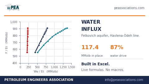
    Fits the Havlena-Odeh straight line to find aquifer size and confirm the Fetkovich model actually applies, instead of assuming a water drive fits without checking. On the built-in example the aquifer carries 117.4 MMstb in place, and it's supplying 87% of the field's pressure support — a field that would misread as depleting fast without this check. Every point a live formula, no macros. Swap in your own field's pressure and production history in a minute.
    image
    Premium  icon
    Download

    Gas Lift Design

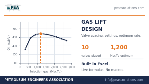
    Spaces gas lift valves down the string and finds the optimum injection rate, instead of stopping at valve placement and leaving rate to guesswork. On the built-in example that's 10 valves placed and a 1,200 Mscf/d optimum — past that point more gas actually costs oil, and the sheet shows exactly where the curve turns over. Every valve a live formula, no macros. Swap in your own well and injection gas in a minute.
    image
    Premium  icon
    Download

    ESP Sizing

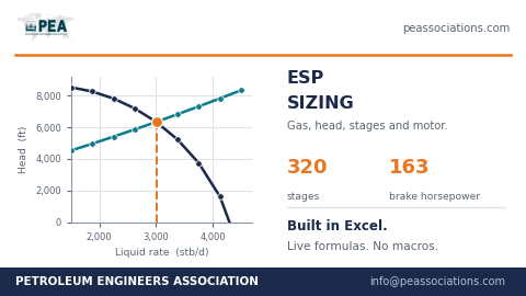
    Sizes an electrical submersible pump against the well's actual duty point — free gas handling, total dynamic head and the pump curve intersecting at the target rate, not a catalog guess. On the built-in example that's 320 stages and 163 brake horsepower at 3,000 stb/d, both a direct read off the head curve. Every stage a live formula, no macros. Swap in your own well and pump curve in a minute.
    image
    Premium  icon
    Download

    Torque & Drag

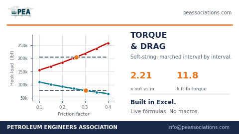
    Marches hook load and torque interval by interval down the trajectory using the soft-string model, instead of one lumped friction estimate for the whole well. On the built-in example hook load tripping out runs 2.21x higher than tripping in, and surface torque reads 11.8 k ft-lb at the working friction factor — both direct reads off the chart as friction factor shifts. Every interval a live formula, no macros. Swap in your own trajectory and mud program in a minute.
    image
    Premium  icon
    Download

    Well Economics

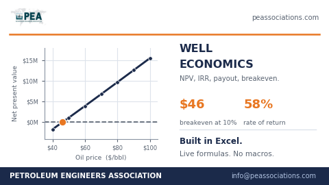
    Prices a single well against oil price, live — NPV, IRR, payout and breakeven all recalculating as the price dial moves. On the built-in example the well breaks even at $46/bbl and returns 58% IRR at today's price, both a direct read off the chart, not a separate model to rebuild. Every term a live formula, no macros. Swap in your own well cost and production profile in a minute.
    image
    Premium  icon
    Download

    Waterflood Pattern Sweep

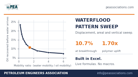
    Predicts waterflood performance from displacement, areal and vertical sweep together, instead of the single-number recovery factor most sheets stop at. On the built-in example only 10.7% of oil is recovered by breakthrough, and switching to polymer flooding lifts that by 1.70x, both a direct read of mobility ratio's grip on sweep. Every term a live formula, no macros. Swap in your own reservoir and fluid data in a minute.
    image
    Premium  icon
    Download

    Pore Pressure & Frac Gradient

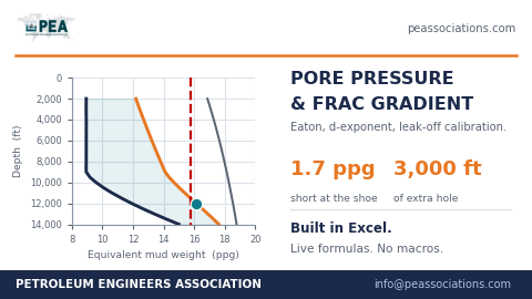
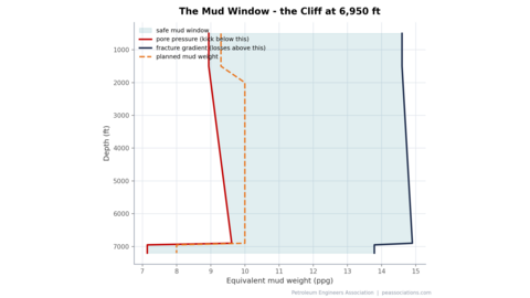
    Predicts pore pressure from the Eaton d-exponent method and fracture gradient in one sheet, then checks whether the casing shoe is actually placed where it needs to be. On the built-in example the shoe sits 1.7 ppg short of margin, leaving only 3,000 ft of hole before the next casing point is forced — a well plan that looks fine on paper until this check runs. Every step a live formula, no macros. Swap in your own drilling data in a minute.
    image
    Premium  icon
    Download

    Choke & Erosional Velocity

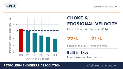
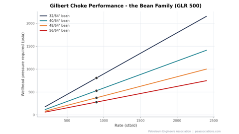
    Sizes a choke for critical flow, then checks it against API RP 14E erosional velocity — two separate constraints most sheets treat as one. Runs four different C factors side by side, and on the built-in example they spread 22% apart on required diameter, with the tightest choke setting running 21% over the erosional limit. Every case a live formula, no macros. Swap in your own rate and pressure conditions in a minute.
    image
    Premium  icon
    Download

    Cement Job Design

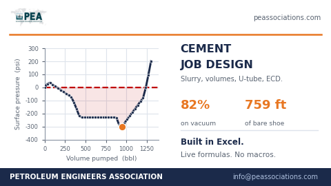
    Tracks surface pressure through a full cement job, U-tube effect and all — the pressure that actually swings negative as heavier cement falls and lighter mud rises on the other side. On the built-in example the well runs on vacuum for 82% of the pumping schedule, and 759 ft of shoe sits bare of cement, both numbers most job sheets never show. Every stage a live formula, no macros. Swap in your own hole and slurry design in a minute.
    image
    Premium  icon
    Download

    Sucker Rod Pumping

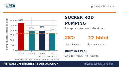
    Sizes a sucker rod pump properly by getting the plunger stroke right — rod stretch and overtravel eat 28% of the surface stroke on the built-in example, and an unanchored tubing loses another 22 bbl/d nobody accounts for. Runs the Goodman diagram against the rod loads so you know the string is actually rated for the duty, not just pumping. Every step a live formula, no macros. Swap in your own well and rod string in a minute.
    image
    Premium  icon
    Download

    Perforating & Completion Skin

    Breaks total skin apart into its five separate causes — perforations, crushed zone, partial penetration, deviation, and formation damage — instead of treating skin as one number with one fix. On the built-in example total skin is 4.3, and none of it is damage, which means acid won't help; the fix is a perforating or deviation change, and the sheet tells you which. Every term a live formula you can trace, no macros. Swap in your own well and completion design in a minute.
    image
    Premium  icon
    Download

    Separator Sizing

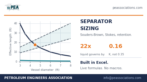
    Sizes a three-phase separator by finding which of two competing jobs actually governs — gas needs area, liquid needs retention volume, and the file finds the crossover instead of assuming it. Both key design constants are derived from first principles, not quoted: Stokes settling comes out at 1.786×10⁻⁶ against the published 1.78×10⁻⁶, and the Souders-Brown K works out to 0.16, not the 0.35 everyone uses — the difference between a real settling calculation and a mist-extractor spec, and it's a 54% swing in vessel size. On the built-in Falcon Field stream (8,000 stb/d oil, 4,000 bwpd, 7.2 MMscf/d) the answer is a 54"×17.7 ft vessel, with the liquid side governing by a factor of 22. Every number a live formula, no macros. Swap in your own stream in a minute.
    image
    Premium  icon
    Download

    Gas Well Deliverability (Four-Point Test)

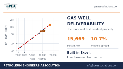
    Runs the classic four-point deliverability test properly — pr²−pwf² plotted on log-log, slope and intercept solved by regression, extended to absolute open flow. On the built-in example it reads 15,669 Mscf/d AOF, with a 10.7% spread flagged between the Rawlins-Schellhardt and LIT methods so you know how much to trust the number. Every point a live formula, no macros. Swap in your own four-rate test data in a minute.
    image
    Premium  icon
    Download

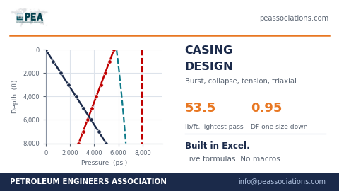
    Casing Design (Burst, Collapse, Tension, Triaxial)

    Runs a casing string against all three loads at once — burst, collapse and tension — plus a triaxial check, not just the single-load pass most sheets stop at. On the built-in example it picks 53.5 lb/ft as the lightest string that passes, and shows the design factor drops to 0.95 one size down, right at the edge of failing. Every load line and pressure profile is a live formula you can trace, no macros. Swap in your own well and mud program in a minute.
    image
    Premium  icon
    Download

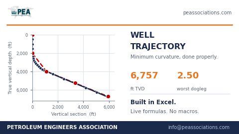
    Well Trajectory (Minimum Curvature)

    Builds a directional well path properly — minimum curvature, not the tangential shortcuts that quietly misplace the bit. On the built-in example the well lands at 6,757 ft TVD with a worst dogleg of 2.50°/100ft, every step a live formula you can trace. No macros. Swap in your own survey stations and it recalculates the whole path in a minute.
    image
    Premium  icon
    Download

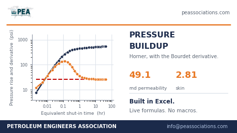
    Pressure Buildup (Horner + Bourdet Derivative)

    Runs a buildup the way it's actually interpreted — Horner semilog plot alongside the Bourdet derivative, so the radial flow stem is confirmed, not assumed. On the built-in example it reads 49.1 md permeability and a skin of 2.81, both live formulas you can click and trace. No macros, no black box. Swap in your own shut-in pressure and time data in a minute.
    image
    Premium  icon
    Download

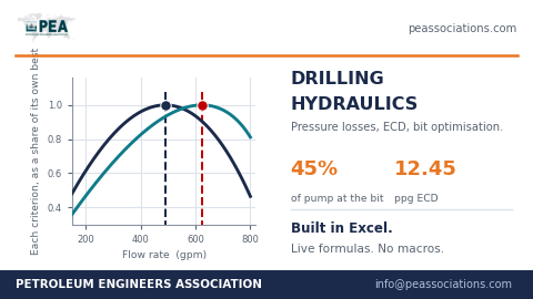
    Drilling Hydraulics

    Optimizes bit hydraulics and tracks ECD in one live sheet — pressure losses split across the whole circulating system, then swept against flow rate to find the nozzle sizing that puts the most horsepower at the bit, not wasted in the string. On the built-in example that's 45% of pump pressure landing at the bit, with ECD holding at 12.45 ppg. No macros, every number a formula you can click and trace. Swap in your own hole geometry and mud program in a minute.
    image
    Premium  icon
    Download

    Well Kill Sheet

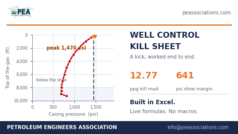
    Shut-in pressures and a pit gain go in; kill mud weight, both circulating pressures, stroke counts and the full drillpipe pressure schedule come out — the sheet a driller actually works to. Identifies the kick type from its own pressure signature — gas, oil or salt water — before anything reaches surface. Solves the part most kill sheets skip: gas rising and expanding, casing pressure computed in closed form at thirteen depths so you see the peak coming before it arrives. Checks the shoe properly too — on the built-in example, peak surface pressure exceeds MAASP and the shoe still holds, with 641 psi to spare, for a reason the sheet explains. Pre-loaded with PEA-9, a 20-bbl gas kick at 10,000 ft — swap in your own well data in a minute. For training, planning and checking, not a replacement for approved operator kill procedures.
    image
    Premium  icon
    Download

    Rate Transient Analysis

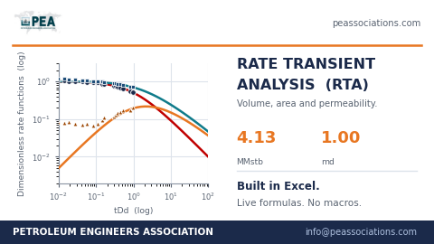
    Solves decline analysis's real limit — real wells don't run at constant flowing pressure — by changing the clock (material balance time), so variable-rate data behaves like constant-rate data. The boundary-dominated stem is exactly harmonic, so the match is done by arithmetic, not by dragging a type-curve overlay and hoping two people get the same answer. Returns what decline analysis can't: drainage volume, drainage area, productivity index and permeability — recovers a planted 1.00 md to within a tenth of a percent on the built-in example. Separates transient from boundary-dominated flow automatically, since fitting one as the other is the most expensive mistake in production analysis. Pre-loaded with PEA-8, two years of daily Falcon Field data through two rate changes — swap in your own well in a minute.
    image
    Premium  icon
    Download

    Flowing Material Balance

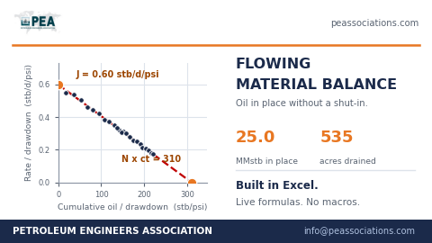
    Gets oil-in-place without shutting the well in — just the rate and flowing pressure the well already reports. One straight line does it all: y-intercept is productivity index, x-intercept gives OOIP times compressibility. Survives what kills decline analysis — the built-in example has the choke opened up halfway through, and both halves still agree to within a fifth of a percent. Turns the volume into a drainage area and radius you can put on a map, so you can see if wells are competing for the same oil. Pre-loaded with PEA-2, Falcon Field (two years of monthly rate and pressure) — swap in your own well in a minute.
    image
    Premium  icon
    Download

    Relative Permeability

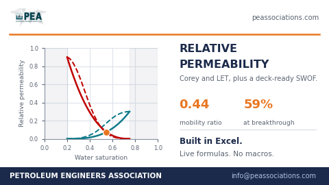
    Set the endpoints and exponents and it builds the curves, the fractional flow they imply, and the recovery they predict — Corey and LET side by side, so you can bend a curve to lab data without losing a defensible form. The Welge tangent is built in, finding flood-front saturation and breakthrough water cut with no calculus and no solver. Ends with a SWOF table that's actually deck-ready — correctly ordered, endpoints exact, capillary pressure capped — copy straight into a simulator. Pre-loaded with Falcon Field sandstone (connate water 0.20, residual oil 0.25) — swap in your own core data in a minute.
    image
    Premium  icon
    Download

    Critical Lift Rate

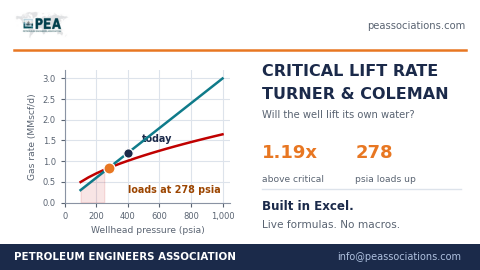
    Computes the gas rate below which a well stops carrying its own water to surface — and how much margin your well has left today. Runs both published methods side by side, Turner and Coleman, which disagree by 20% on the same well, and shows which one applies at your pressure. Answers the real question — at what wellhead pressure will this well load up — and prices the fix, six standard tubing strings sized against your expected rate. Pre-loaded with PEA-6, a Falcon Field gas well at 400 psia making 1.2 MMscf/d with water — swap in your own well in a minute.
    image
    Premium  icon
    Download

    RFT/MDT Pressure Analysis

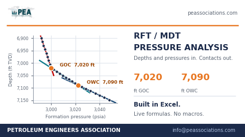
    Paste your formation-tester depths and pressures and it fits a gradient line to each fluid, turns the slope into a density, and reports the gas-oil and oil-water contacts to the foot — by least squares, not dragged by eye. Checks itself three ways: gradients against published fluid bands, each station against its own line, and oil density against your PVT (accurate to a quarter degree API on the built-in example). Also prices the uncertainty — how far a contact moves if a gradient is off by a hundredth of a psi per foot. Pre-loaded with PEA-4, a 24-station Falcon Field appraisal run through gas cap, oil column and aquifer — swap in your own run in a minute.
    image
    Premium  icon
    Download

    PVT Correlations

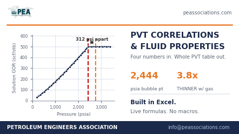
    Give it oil gravity, gas gravity, solution GOR and temperature — four numbers — and it builds the whole fluid table: bubble point, Rs, Bo, Bt, oil and gas viscosity, z-factor and Bg at every pressure you need. All explicit correlations, no solver, so it recomputes instantly when you change a number. Shows bubble point two ways, Standing and Vazquez-Beggs, because they disagree by 13% on the built-in fluid and most engineers never check that. Charts the signature shapes — Bo peaking and viscosity bottoming out right at the bubble point — so you can see if your table is behaving. Pre-loaded with Falcon Field oil (32° API, 500 scf/stb, 180°F) — swap in your own fluid in a minute.
    image
    Premium  icon
    Download

    Nodal Analysis (IPR + VLP)

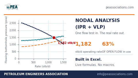
    Finds where a well actually flows — the crossing of what the reservoir delivers and what the tubing can carry. Runs a real 8-segment outflow march down the tubing, with gas breaking out of solution and friction handled properly, not one lazy average gradient. Compares three tubing sizes side by side plus a wellhead-pressure trade, each a full re-run of the whole well. Ends where it matters: how much rate a tubing change actually buys, and how much of the well's potential you're currently using. Pre-loaded with PEA-2, Falcon Field (7,000 ft oil well, 2-7/8" tubing) — swap in your own well in a minute.
    image
    Premium  icon
    Download

    Volumetrics & Reserves

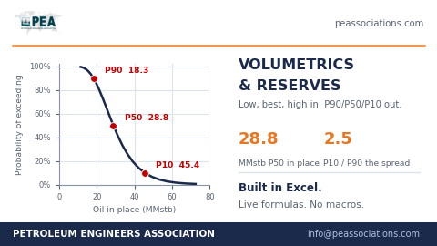
    Give each input a low, best and high estimate and it returns the full range — P90, P50, P10, the mean, and the S-curve behind them — no Monte Carlo, no macro, just log-space arithmetic done properly. Tells you which input is actually costing you certainty, with a variance ranking and swing chart showing where an appraisal well or better seismic would pay for itself. Recoverable volume carries the recovery factor's own uncertainty too, so the P90 you quote is a real P90. Pre-loaded with a Falcon Field appraisal example (640-acre Gulf Coast sandstone) — swap in your own prospect in a minute.
    image
    Premium  icon
    Download

    Gas Material Balance (p/z)

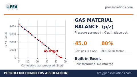
    Type in your field's production and pressure history and it draws the classic p/z line, extends it to zero, and reads off the gas in place — the oldest and most trusted measurement in gas reservoir engineering. Z-factor computed automatically by Papay's correlation, but the yellow cell is open for your own lab values. Runs the water-drive check most spreadsheets skip, catching a pressure-supported pool before it lies to you on the plot. Pre-loaded with a real worked example (Falcon Field dry-gas pool, ten pressure surveys, 31.9 Bscf produced) — swap in your own field in a minute.
    image
    Premium  icon
    Download

    Decline Curve Analysis & Reserves

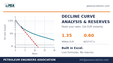
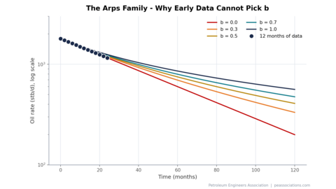
    Paste your own monthly production rates into the yellow column and it fits an Arps decline for you — 30 trial b-values solved by least squares, the best one picked in the open, returning EUR, remaining reserves and years left. Built-in terminal-decline switch stops hyperbolic forecasts from promising oil forever, and the economic limit is computed from your price and cost inputs, not assumed. Shows the uncertainty most tools hide: if your data can't tell b = 0.55 from b = 0.65, this sheet says so and prices both. Comes pre-loaded with a 36-month worked example (PEA-2, Falcon Field) — replace it with your own well in under a minute.
    image
    Premium  icon
    Download

    Petrophysics — Expert-Edition Master Workbook

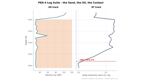
    A real 22-level log suite runs the whole book — gamma ray, density, neutron and resistivity in proper depth tracks — as you build shale volume, porosity from logs, Archie's saturation from first principles, the Pickett plot, shaly-sand Simandoux, and full rock typing (RQI, FZI, Winland R35) with permeability predicted and audited against core. Ends in cutoffs and net pay for a real 96-ft interval with an oil leg, a shaly streak, a tight zone and a water contact. Honest throughout — Archie's shaly-sand bias is computed level by level, not hidden. Built for training rooms, company induction, and petrophysicists' and geologists' daily CPI work.
    image
    Premium  icon
    Download

    Reservoir Engineering Fundamentals — Expert-Edition Master Workbook (Flagship Sample Volume)

    One well, one field, every reservoir engineering fundamental connected in live formulas — porosity, permeability, capillary pressure, PVT, volumetrics, radial flow, well testing, pressure buildup, material balance and decline curves. The Horner engine centrepiece recovers permeability, skin and p* straight from raw shut-in gauge data. Every big number is cross-checked two ways — core permeability vs. well-test permeability, volumetric OOIP vs. material-balance OOIP — and they agree, live. Built for training rooms, company induction, and working engineers' daily sanity checks on real field decisions.
    image
    Premium  icon
    Download

    Petroleum Production Engineering — Expert-Edition Master Workbook

    The complete production system built live from IPR to the Xmas tree — a Vogel inflow curve, a 176-cell segmented pressure-traverse engine marching every rate down 7,000 ft of tubing for two tubing sizes, and the classic IPR-VLP nodal crossing that decides the well's real rate (1,715 vs 1,959 stb/d, not a guess). Covers choke sizing, wellhead and Xmas tree rating, flow assurance, and an artificial lift preview, all fed by 14 live charts. Honestly convicts the common shortcuts too — the single-average-pressure method is shown losing 477 psi of accuracy, right next to the method that doesn't. Built for training rooms, company induction, and production engineers' daily surveillance and completion decisions.
    image
    Premium  icon
    Download

    Reservoir Simulation in a Spreadsheet — Expert-Edition Master Workbook

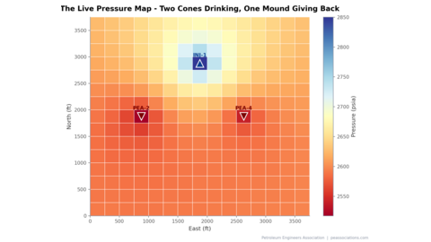
    A live 15x15 pressure map of the Falcon Field block, built cell by cell from real transient physics — two producers pulling down pressure, an injector raising a mound, all redrawn as you turn the time dial from 1 day to 1 year. Includes a real finite-difference engine (20 blocks, 36 timesteps) that you can deliberately push past its stability limit to see a simulation go unstable — one of the most memorable lessons in numerical modeling. A balance audit shows exactly how much pressure leaks through the edges of any finite model, and the book ends by scoring three drilling locations straight off the live map. Built for training rooms, company induction, and reservoir engineers meeting their first simulator.
    image
    Premium  icon
    Download

    Drilling Engineering — Expert-Edition Master Workbook

    A complete well plan built from the mud window to the kill sheet — pressure windows, casing seat selection, mud design, hydraulics, well control, drillstring loads, bit economics and cementing, all in live formulas across 15 publication-grade charts. The centrepiece is a real kick worked start to finish: shut-in pressures become kill mud weight, pump schedule and the classic declining drillpipe-pressure line, exactly as it's used on a rig floor. Drilled through a depleted reservoir zone that squeezes the mud window and dictates casing depth — every dollar and every psi computed, not assumed. Built for training rooms, company induction, and drilling and wellsite engineers' daily work.
    image
    Premium  icon
    Download

    Petroleum Economics & Field Development — Expert-Edition Master Workbook

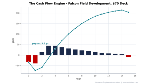
    A live cash flow engine that prices a full 6-well, $126M Falcon Field development from first barrel to final verdict — NPV, IRR, payout, all computed cell by cell across sixteen years. Turn the oil price dial between $50, $70 and $90 and watch the whole book, including a tornado sensitivity ranking and a resilience console, repaint instantly. Two real capital decisions — a workover vs. an infill well — are priced incrementally, the way brownfield dollars actually get approved. Includes CAPEX planning, OPEX modeling, fiscal terms, and a full worked example with live dashboard. Built for engineers facing their first AFE, training rooms, and anyone who signs, defends or challenges a development budget.
    image
    Premium  icon
    Download

    Well Test Type-Curve Atlas — Expert-Edition Master Workbook

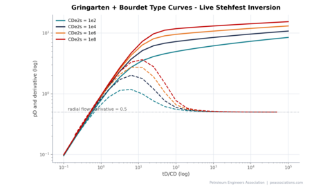
    A hands-on Excel workbook that teaches pressure transient analysis from first principles — no pasted curves, no black boxes. Build the Bourdet derivative, run a live Stehfest-inversion Laplace engine (Gringarten & Bourdet type curves computed in cells you can click), match a real 150-hour PEA-5 buildup, cross-check with semilog analysis, and locate a sealing fault at 718 ft. Includes the signature gallery of seven classic derivative shapes, a dual-porosity primer, common interpretation failures explained, and a full worked example with live dashboard. Built for training rooms, company induction, and real well test interpretation work.
    logo
    GET IN TOUCH

    PETROLEUM ENGINEERS ASSOCIATION
    JHARKHAND, INDIA

    Contact : +91 6205464268
    Email: info@peassociations.com

    Tax Registration Number:
    20DIGPA7260B1Z1

    COMPANY
    About Us Contact Us Articles Download Certificate
    Become an instructor One on one mentorship Gallery Testimonials Feedback
    logo
    Payment Terms Privacy Policy Terms of Use Sitemap Cookie Preferences Security
    © 2026 Petroleum Engineers Association. All Right Reserved.
    Design & Developed By Bitstreaks Company Logo
    WhatsApp Whatsapp icon
    Let us know how we can assist you? logo
    Let us know how we can assist you? ✖

    PEA uses cookies and other tracking technologies to improve your browsing experience for the following purposes: to enable basic functionality of the website, to provide a better experience on the website, to measure your interest in our products and services and to personalize marketing interactions, to deliver ads that are more relevant to you.

    Change my preferences